2 From corpora to clouds

The main goal of the methodological framework presented here is to explore semasiological structure from textual data. The starting point is a corpus, i.e. a selection of texts, and one of the most tangible outputs is what we will call clouds: the visual representation of textual patterns as dense areas in a 2d scatterplot. In this chapter we will explain how to generate clouds from the raw, seemingly indomitable ocean of a corpus.

First, we will describe how token-level vector space models are created: these are mathematical representations of the occurrences of a lexical item. We will focus on context-counting models, but this is by no means the only viable path. Other techniques, such as BERT (Devlin et al. 2019)⁴, that can also generate vectors for individual instances of a word, could be used for the first stage of this workflow. Section 2.1 will describe the process and the rationale without assuming a strong mathematical background for the reader, leaving the deeper technicalities to Section 2.2. In Section 2.3, we will break apart the workflow into the multiple choices that the researcher needs to make and that result in a potentially infinite number of models, while Section 2.4 briefly presents a method to select a few representative models. Finally, Section 2.5 summarizes the chapter.

2.1 A cloud machine

At the core of vector space models, aka distributional models, we find the Distributional Hypothesis, which is often linked to Harris’s observation that “difference of meaning correlates with difference of distribution” (1954: 156), but also to Firth’s “You shall know a word by the company it keeps” (1957: 11) and Wittgenstein’s “the meaning of a word is its use in the language”⁵ (1958: 20). In other words, items that occur in similar contexts in a given corpus will be semantically similar, while those that occur in different contexts will be semantically different (Jurafsky & Martin 2020, Ch. 6; Lenci 2018). Crucially, this does not imply that we can describe an individual item with their distributional properties, but that comparing the distribution of two items can tell us something about their semantic relatedness (Sahlgren 2006: 19).

Firth (1957) inspired generations of corpus linguists to look at collocations as part of the semantic description of a lemma. The Birmingham school, pioneered by John Sinclair, used co-occurrence frequency information to describe a lexical item by the set of those context words most attracted to them. Due to the skewed distribution of word frequencies, known as Zipf’s law, this attraction cannot be measured in terms of raw co-occurrence frequencies. For example, the most frequent lemma in the (Dutch) corpus used for this research, discarding punctuation, is de ‘the (fem./masc.),’ which occurs 28.1 million times. The second most frequent lemma, van ‘from,’ occurs 12.6 milion times, and it is followed by het ‘the (neutral)’ and een ‘a, an,’ with corresponding frequencies of 11.7 and 11.1 million times each. For every 100 words in the corpus, excluding punctuation, \(14\) are one of these four words. Of the total of 4.6 million different words, 61% are hapax legomena, i.e. they occur once, and 172 lemmas cover 50% of all the occurrences. As a consequence, co-occurrences with very frequent words are not as informative as those with less frequent words, and hence raw co-occurrence frequencies are transformed to measures of association strength, such as mutual information (see Section 2.2.1) or t-score, among others (for an overview see Evert 2009; Gablasova, Brezina & McEnery 2017). In collocational studies, researchers typically set a threshold of association strength and only look at the context words that surpass it.

At their core, context-counting vectors are lists of association strength values. Each word is represented by its association strength to a long array of words that it might co-occur with, as shown in Table 2.1. Unlike in collocation studies, low values — or even lack of co-occurrence — are not excluded, but used in the comparison with other words that might. Going back to the Firthian motto, a collocational study would describe me with the list of people that I talk to the most, whereas a distributional model would compare me to someone else based on who either of us talks to and how often we talk to them. The more people we have in common, the more similar we are, but people that neither of us talks to have no impact on the comparison.

Table 2.1 shows small vectors representing the English nouns linguistics, lexicography, research and chocolate, as well as the adjective computational, with co-occurrence information obtained from the GloWbE (Global Word-based English) corpus. The values are their association strength pmi with each of the lemmas in the columns: the higher the values, the stronger the attraction between the word in the row and the word in the column (See Section 2.2.1). From a collocational perspective, linguistics is strongly attracted to both language and English, i.e. they occur very often in a span of 10 words from each other, considering their individual frequencies; it is less attracted to word and to speak, and does not co-occur with either to eat or Flemish within that window, in this corpus.

Table 2.1: Small example of type-level vectors, with pmi values based on a symmetric window of 10. Frequency data extracted from GloWbE.

target	language/n	word/n	flemish/j	english/j	eat/v	speak/v
linguistics/n	4.37	0.99		3.16		0.41
lexicography/n	3.51	2.18		2.19		2.09
computational/j	1.6	0.08		-1		-1.8
research/n	0.2	-0.84	0.04	-0.5	-0.68	-0.38
chocolate/n	-1.72	-0.53	1.28	-0.73	3.08	-1.13
Note:
Part-of-speech is indicated after a slash: n = noun, j = adjective, v = verb

Each row in Table 2.1 is a vector coding the distributional information of the lemma it represents. By lemma we refer to the combination of a stem and a part of speech, e.g. chocolate/n covers chocolate, chocolates, Chocolate, etc. These vectors are meant to code the distributional behaviour of the linguistic forms they represent — in this case lemmas —, in order to operationalize the notion of distributional similarity and, consequently, model their meaning. For example, in Table 2.1 the first two rows, representing linguistics and lexicography, are similar to each other: both words have a similar attraction to language and to English, even if the values for word and to speak are more different. More importantly, they are more similar to each other than to other rows in the table, which have lower values for those four columns and might even co-occur with Flemish and to eat as well. The Distributional Hypothesis expresses the observation that words that are distributionally similar, like linguistics and lexicography, are semantically similar or related, whereas words that are distributionally different, like linguistics and chocolate, are semantically different or unrelated.

The rows in this table are type-level vectors: each of them aggregates over all the attestations of a given lemma in a given corpus to build an overall profile. As a result, it collapses the internal variation of the lemma, i.e. its different senses or semasiological structure. In order to uncover such information, we need to build vectors for the individual instances or tokens, relying on the same principle: items occurring in similar contexts will be semantically similar. For instance, we might want to model the three (artificial) occurrences of study in (1) through (3), where the target item is in bold and some context words are in italics.

1. Would you like to study lexicography?
2. They study this in computational linguistics as well.
3. I eat chocolate while I study.

Given that, at the aggregate level, a word can co-occur with thousands of different words, type-level vectors can include thousands of values. In contrast, token-level vectors can only have as many nonzero values as the individual window size comprises, which drastically reduces the chances of overlap between vectors. In fact, the three examples don’t share any item other than the target. As a solution, inspired by Schütze (1998), (a selection of) the context words around the token is replaced with their respective type-level vectors (Heylen, Speelman & Geeraerts 2012; Heylen et al. 2015; De Pascale 2019). Concretely, example (1) is represented by the vector for its context word lexicography, that is, the second row in Table 2.1; example (2) by the sum of the vectors for linguistics (row 1) and computational (row 3); and example (3) by the vector for chocolate (row 5). This not only solves the sparsity issue, ensuring overlap between the vectors, but also allows us to find similarity between (1) and (2) based on the similarity between the vectors for lexicography and linguistics. As we will see in Section 2.3, we can even use the association strength between the context words and the target type, i.e. to study, and give more weight to the context words that are more characteristic of the lemma we try to model. The result of this procedure is a co-occurrence matrix like the one shown in Table 2.2. Each row represents an instance of the target lemma, e.g. to study, and each column, a lemma occurring in the corpus⁶; the values are the (sum of the) association strength between the words that occur around the token, i.e. their first-order context words, and each of the words in the columns, i.e. the second-order context words. In addition, all negative and missing values value have been set to zero, due to the unreliability of negative pmi values (see Section 2.2.1).

Table 2.2: Small example of token-level vectors of three artificial instances of to study.

target	language/n	word/n	english/j	speak/v	flemish/j	eat/v
study\(_1\)	4.37	0.99	3.16	0.41	0.00	0.00
study\(_2\)	5.97	1.07	2.16	0.00	0.00	0.00
study\(_3\)	0.00	0.00	0.00	0.00	1.28	3.08

The next step in the workflow is to compare the items to each other. We can achieve this by computing cosine distances between the vectors (see Section 2.2.2 for the technical description). The resulting distance matrix, shown in Table 2.3, tells us how different each token is to itself, which takes the minimum value of 0, and to each of the other tokens, with a maximum value of 1. We can see that (1) and (2) are very similar to each other, because they co-occur with similar context words, i.e. linguistics and lexicography, but drastically different from (3), which was modelled based on chocolate. The specific selection of context words is crucial: if we had selected computational but not lexicography to model (2), it would have resulted in a larger difference with (1). The series of choices that we can make and that have been made for this research project are discussed in Section 2.3.

Table 2.3: Cosine distance matrix between the three artificial instances of to study.

	study\(_1\)	study\(_2\)	study\(_3\)
study\(_1\)	0.00	0.04	1
study\(_2\)	0.04	0.00	1
study\(_3\)	1.00	1.00	0

Table 2.3 is small and simple, but what if we had hundreds of tokens? The more items we compare to one another, the larger and more complex the distance matrix becomes. In order to interpret it, we need more stages of processing. On the one hand, dimensionality reduction techniques such as mds, t-sne and umap, which will be discussed in Section 2.2.3, offer us a way of visualizing the distances between all the models by projecting them to a 2d space. We can then represent each model into a scatterplot, like in the plots of Figure 2.1, where each point represents a token, and their distances in 2d space approximate their distances in the multidimensional space of the co-occurrence matrix. Visual analytics, such as the tool described in Chapter 3, can then help us explore the scatterplot to figure out how tokens are distributed in space, why they form the groups they form, etc.

Word Sense Disambiguation makes use of clustering algorithms to extract clusters of similar tokens from their models. The idea behind it is that, if distributional similarity correlates with semantic similarity, groups of similar tokens should share the same sense and have a different sense from other groups of tokens. In Chapter 6 we will see to what degree this assumption holds in this data and with these methods.

The final step in our workflow is, then, the combination of dimensionality reduction and clustering, which results in the right plot of Figure 2.1: by means of dimensionality reduction, tokens are located in a scatterplot so that distributional similarities are approximated as spatial similarities, and groups of similar tokens are assigned different colours. In previous research, which did not integrate clustering procedures in this manner, the term cloud was used to refer to a full model (Heylen et al. 2015; Wielfaert et al. 2019; De Pascale 2019; Montes & Heylen 2022). In this study, instead, cloud will refer to each of the clusters, identified by colours in the scatterplot.

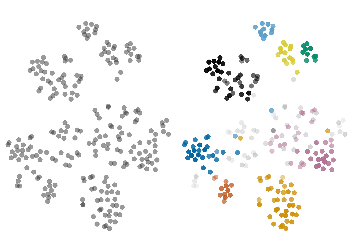
Figure 2.1: 2d representation of Dutch hachelijk ‘dangerous/critical.’

2.2 The chemistry of cloud making

A typical vector space model is an item-by-feature matrix: its rows code items, its columns code features, and its cells code information related to the frequency with which the items and features co-occur. The first distributional models counted the occurrences of words in documents and represented them in word-by-document matrices; the models described here are token-by-feature matrices, in which the rows are attestations of a lexical item and the features are second-order co-occurrences, i.e. context words of the context words of the token. Turney & Pantel (2010) offer an overview of different kinds of matrices, based on the items modelled and the features used to describe them. Besides matrices, vector space models can be tensors, which are generalisations of matrices for more dimensions and can allow for more complex interactions, e.g. subject-verb-object triples in Van de Cruys, Poibeau & Korhonen (2013); see also Lenci (2018).

Models can be based on co-occurrence counts, as is the case in these studies, or on machine-learning algorithms trained to predict the context around a word or fill in an empty slot given a few words around it. These context-predicting models use the weights of their neural networks as features in the vectorial representations of the words they predict. A number of papers have explored which kind of models work best for different tasks, with uncertain results (Baroni, Dinu & Kruszewski 2014; Levy, Goldberg & Dagan 2015). As explained before, such context-predicting models will not be explored in this dissertation, although their integration would be interesting for further avenues of research.

The workflow described in the previous section relies on mathematical principles to obtain linguistic patterns from a (mostly) raw corpus. A full understanding of the formulae that underlie each step is not necessary to grasp the gist of this methodology, but it is required for an appropriate implementation. In this section, we will take a deeper look into the technical aspects the machinery behind the process, in particular association strengths, similarity metrics, dimensionality reduction techniques and clustering algorithms.

2.2.1 Association strength: PMI

The distribution of words in a corpus follows a power law: a few items are extremely frequent, and most of the items are extremely infrequent. Association measures transform raw frequency information to measure the attraction between two items while taking into account the relative frequencies with which they occur. They typically manipulate, in different ways, the frequency of the node \(f(n)\), the frequency of its collocate \(f(c)\), their frequency of co-occurrence \(f(n,c)\) and the size of the corpus \(N\). Evert (2009) and Gablasova, Brezina & McEnery (2017) offer an overview of how different measures are computed and used in corpus linguistics; Kiela & Clark (2014) compare measures used in distributional models.

In the studies discussed here, I will only use (positive) pointwise mutual information, or (p)pmi (Church & Hanks 1989), one of the most popular measures both in collocation studies and distributional semantics (Bullinaria & Levy 2007; Kiela & Clark 2014; Jurafsky & Martin 2020; Lapesa & Evert 2014). Its formula is shown in equation (2.1), where \(p(n) = \frac{f(n)}{N}\), i.e. the proportion of occurrences in the corpus that correspond to \(n\).

\[\begin{equation} I(n, c) = \log \frac{p(n,c)}{p(n)p(c)} = \log \left( \frac{f(n,c)}{f(n)f(c)} N \right) \tag{2.1} \end{equation}\]

Negative pmi values tend to be unreliable, so positive pmi or ppmi is used, in which the negative pmi values are turned to zeros (Bullinaria & Levy 2007; Kiela & Clark 2014; De Pascale 2019; Jurafsky & Martin 2020: 109). Furthermore, pmi is known for its bias towards infrequent events: when either \(p(n)\) or \(p(c)\) is very low, pmi tends to be very high. In collocation studies, this bias may be counteracted by combining pmi filters with other measures that favour frequent co-occurrences, such as t-scores or log-likelihood ratio (McEnery, Xiao & Tono 2010). In distributional semantics, the accuracy of models that rely on ppmi seems not to be affected by the issue presented by this bias; moreover, in these studies any lemma with \(f(n) < 217\), i.e. occurring less than once every two million tokens, was excluded, to avoid too sparse, uninformative vectors.

2.2.2 Similarities and distances: cosine

After obtaining the token-by-feature matrices, the distances between the vectors must be computed. Typically, the implementations for the dimensionality reduction and clustering can take the item-by-feature matrices as input and compute the distances under-the-hood, but they do not necessarily offer the option of computing our distance measure of choice, cosine.

Cosine is a measure of similarity between vectors \(\mathbf{v}\) and \(\mathbf{w}\) and is defined in equation (2.2); it coincides with the normalised dot product of the vectors (Jurafsky & Martin 2020: 105).

\[\begin{equation} \mathrm{cosine}(\mathbf{v}, \mathbf{w}) = \frac{\mathbf{v} \cdot \mathbf{w}}{\left|\mathbf{v}\right|\left|\mathbf{w}\right|} = \frac{\sum\limits_{i=1}^N v_iw_i}{\sqrt{\sum\limits_{i=1}^N v_i^2}\sqrt{\sum\limits_{i=1}^N w_i^2}} \tag{2.2} \end{equation}\]

For positive values, e.g. when using ppmi, the cosine similarity ranges between 0 and 1: it will be 1 between identical vectors and 0 for orthogonal vectors, which do not share nonzero dimensions, like study\(_1\) and study\(_3\) in Table 2.2. Cosine is sensitive to the angle between the vectors, and not to their magnitude: the similarity between study\(_1\) and a vector created by multiplying all the cells in study\(_1\) by any constant will still be 1.

Cosine similarity is the most common metric in distributional models (Jurafsky & Martin 2020: 105) and has been shown to outperform other measures, especially when combined with ppmi (Kiela & Clark 2014; Lapesa & Evert 2014; Bullinaria & Levy 2007)⁷. One of the ways in which it is used is for semantic similarity tasks: the nearest neighbours of an item are extracted, by selecting the vectors with highest cosine similarity to the target vector. In these studies, similarities are usually transformed to distances by inverting the scale (\(\mathrm{cosine}_{\mathrm{dist}} = 1- \mathrm{cosine}_{\mathrm{sim}}\)), so that identical vectors — and each vector to itself — have a cosine distance of 0 and orthogonal vectors have a cosine distance of 1, as shown in Table 2.3.

Before applying dimensionality reduction or clustering algorithms, the cosine distances were further transformed with the aim of giving more weight to short distances, i.e. nearest neighbours, and decreasing the impact of long distances. For each token vector \(\mathbf{v}\) with \(n\) dimensions, we define the transformed vector \(\mathbf{v}_{\mathrm{transformed}}\) as \(\mathbf{v}_{\mathrm{transformed}_i} = \log (1 + \log rank(\mathbf{v})_i)\) for each \(i\), with \(1 \le i \le n\), and where \(rank(\mathbf{v})_i\) is the similarity rank of the \(i\)th value in \(\mathbf{v}\). For example, if originally we have the distances \(\mathbf{v} = [0, 0.2, 0.8, 0.3]\), the rank transformation returns \(rank(\mathbf{v}) = [1, 2, 4, 3]\), which after the first logarithm transformation becomes \([0, 0.693, 1.39, 1.099]\) and, after the second transformation, \(\mathbf{v}_{\mathrm{transformed}} = [0, 0.52, 0.86, 0.74]\). On the one hand, the magnitude of the distance is not as important as its ranking among the nearest neighbours. On the other, the lower the ranking, the smaller the impact: the difference between the final values for ranks 1 and 2 is larger than between ranks 2 and 3. The new matrix, where each row \(\mathbf{v}\) has been replaced with its \(\mathbf{v}_{\mathrm{transformed}}\), is converted to euclidean distances.

While cosine distances are used to measure the similarity between token-level vectors, euclidean distances will be used to compare two vectors of the same token across models, and thus compare models to each other. Concretely, let’s say we have two matrices, \(\mathbf{A}\) and \(\mathbf{B}\), which are two models of the same sample of tokens, built with different parameter settings, and we want to know how similar they are to each other, i.e. how much of a difference those parameter settings make. Their values are already transformed cosine distances. A given token \(i\) has a vector \(\mathbf{a}_i\) in matrix \(\mathbf{A}\) and a vector \(\mathbf{b}_i\) in matrix \(\mathbf{B}\). For example, \(i\) could be example (2) above, and its vector in \(\mathbf{A}\) is based on the co-occurrence with computational and linguistics, as shown in Table 2.2, while its vector in \(\mathbf{B}\) is only based on computational. The euclidean distance between \(\mathbf{a}_i\) and \(\mathbf{b}_i\) is computed with the formula shown in equation (2.3). After running the same comparison for each of the tokens, the distance between the models \(\mathbf{A}\) and \(\mathbf{B}\) is then computed as the mean of those tokenwise distances across all the tokens modelled by both: \(d(\mathbf{A},\mathbf{B}) = \frac{\sum_{i=1}^nd(\mathbf{a}_i, \mathbf{b}_i)}{N}\). Alternatively, the distances between models could come from procrustes analysis⁸, like Wielfaert et al. (2019) do, which has the advantage of returning a value between 0 and 1. However, this method is much faster and returns comparable results.

\[\begin{equation} d(\mathbf{a}_i, \mathbf{b}_i) = \sqrt{\sum\limits_{i=j}^n(a_j-b_j)^2} \tag{2.3} \end{equation}\]

2.2.3 Dimensionality reduction for visualization: t-SNE

Dimensionality reduction algorithms try to reduce the number of dimensions of a high-dimensional entity while retaining as much information as possible. In distributional models, they have two main applications: one that reduces thousands of dimensions to a few hundred, and one that reduces them to only two.

The first application of dimensionality reduction, with techniques like svd (Singular Value Decomposition), is meant to deal with the sparsity of high-dimensional vectors. Due to the frequency distribution discussed above, many words never occur in the vicinity of each other, resulting in many zeros in their context-counting representations and therefore inflated differences between the vectors. In particular, techniques like Latent Semantic Analysis (Landauer & Dumais 1997) are based on the observation that the dimensions obtained from this process are semantically interpretable. It could also be used for token-level spaces, but the comparisons discussed in De Pascale (2019: 246) indicate that they don’t necessarily perform better than non reduced spaces. Both dimensionality reduction techniques and neural networks are suggested as ways of condensing very long, sparse vectors (Jurafsky & Martin 2020; Bolognesi 2020). We will not go into the technical aspects because these techniques have not been implemented in the studies described here. Instead, we have compared vectors of different lengths based on other selection methods for the second-order features. Combining them with svd is a possible avenue for future comparisons.

The second application of dimensionality reduction is used for visualization purposes. A token-by-feature matrix can be understood as a multidimensional space: each of the columns is a dimension of space and the values of cells are the coordinates of the items in each of these dimensions. That is why we can use cosine distances, which measures angles: if we draw a vector from the origin (zero in all dimensions) to the point with those coordinates, it diverges from other vectors with a given angle that grows wider as the vectors diverge, leading to larger cosine distances. We can mentally picture or even draw positions, vectors and angles in up to 3 dimensions, but distributional models have hundreds if not thousands of dimensions. These applications of dimensionality reduction, then, are built to project the distances between items in the multidimensional space to euclidean distances in a low-dimensional space that we can visualize. The different implementations can receive the token-by-feature matrix as input, but will not typically compute cosine distances between the items, so the distance matrix is provided as input instead. The literature tends to go for either multidimensional scaling (mds) or t-stochastic neighbour embeddings (t-sne); recently, an interesting alternative called umap has been introduced, which I’ll discuss shortly.

The first option, mds, is an ordination technique, like principal components analysis (pca). It has been used for decades in multiple areas (e.g. Cox & Cox 2008); its most relevant application for this case, non-metric multidimensional scaling, was developed by Kruskal (1964). It tries out different low-dimensional configurations aiming to maximize the correlation between the pairwise distances in the high-dimensional space and those in the low-dimensional space: items that are close together in one space should stay close together in the other, and items that are far apart in one space should stay far apart in the other. The output from mds can be evaluated by means of the stress level, i.e. the complement of the correlation coefficient: the smaller the stress, the better the correlation between the measures. Unlike pca, however, the dimensions are not meaningful per se; two different runs of mds may result in plots that mirror each other while representing the same thing. Nonetheless, the R implementation vegan::metaMDS() (Oksanen et al. 2020) rotates the plot so that the horizontal axis represents the maximum variation. In cognitive linguistics literature both metric (Koptjevskaja-Tamm & Sahlgren 2014; Hilpert & Correia Saavedra 2017; Hilpert & Flach 2020) and non-metric mds (Heylen, Speelman & Geeraerts 2012; Heylen et al. 2015; Perek 2016; De Pascale 2019) have been used.

The second technique, t-sne (van der Maaten & Hinton 2008; van der Maaten 2014), has also been incorporated in cognitive distributional semantics (Perek 2018; De Pascale 2019). It is also popular in computational linguistics (Smilkov et al. 2016; Jurafsky & Martin 2020); in R, it can be implemented with Rtsne::Rtsne() (Krijthe 2018). The algorithm is quite different from mds: it transforms distances into probability distributions and relies on different functions to approximate them. Moreover, it prioritises preserving local similarity structure rather than the global structure: items that are close together in the high-dimensional space should stay close together in the low-dimensional space, but those that are far apart in the high-dimensional space may be even farther apart in low-dimensional space. Compared to mds, we obtain nicer, tighter clouds (see Figure 2.2), but the distance between them is less interpretable: even if we trust that tokens that are very close to each other are also similar to each other in the high-dimensional space, we cannot extract meaningful information from the distance between these groups.

In addition, it would seem that points that are far away in a high-dimensional space might show up close together in the low-dimensional space (Oskolkov 2021). In contrast, Uniform Manifold Approximation and Projection, or umap (McInnes, Healy & Melville 2020), penalizes this sort of discrepancies. It would be an interesting avenue for further research, but a test on the current data did not reveal substantial improvements between t-sne and umap that would warrant the replacement of the technique within the duration of this project (see Figure 2.2 for an example with default parameters. In other models, differences include longer shapes). Other known advantages such as increased speed were not observed in the small samples under consideration — in fact, the R implementation of umap (Konopka 2020) was even slower.

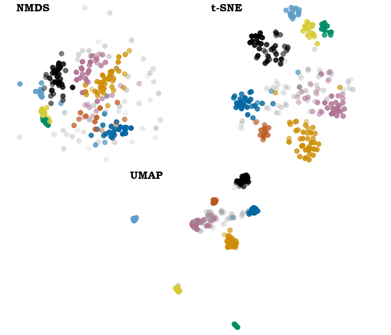
Figure 2.2: Two 2d representations of the same model of hachelijk ‘dangerous/critical’: bound5all-ppmiweight-focall. Non-metric mds on the top left, t-sne to its right and umap at the bottom. Colours indicate hdbscan clusters.

Unlike mds, t-sne requires setting a parameter called perplexity, which roughly indicates how many neighbours the preserved local structure should cover. Low values of perplexity lead to numerous small groups of items, while higher values of perplexity return more uniform, round configurations (Wattenberg, Viégas & Johnson 2016). I have explored perplexity values of 10, 20, 30 and 50, and for this dataset 30 — the default value in the R implementation — has proved to be the most stable and meaningful. Unless otherwise stated, the figures in this text — including Figure 2.1 — will illustrate t-sne token-level representations with perplexity of 30. To represent distances between models, instead, non-metric mds is used (only in Section 3.2).

For both mds and t-sne we need to state the desired number of dimensions before running the algorithm — for visualization purposes, the most useful choice is 2. Three dimensions are difficult to interpret if projected on a 2d space, such as a screen or paper (Card, Mackinlay & Shneiderman 1999; Wielfaert et al. 2019). As we mentioned before, the dimensions themselves are meaningless, hence no axes or axis ticks will be included in the plots. However, the scales of both coordinates are kept fixed: given three points \(a=(1, 1.5)\), \(b=(1, 0.5)\) and \(c=(0, 1.5)\), the distance between \(a\) and \(b\) (1 unit along the \(x\)-axis) will be the same as the distance between \(a\) and \(c\) (1 unit along the \(y\)-axis).

2.2.4 Clustering: HDBSCAN

In word sense disambiguation tasks, the vectorial representations of different attestations are clustered into groups of similar tokens. There is a variety of clustering algorithms, appropriate for different kinds of data and structures. I will not offer an overview of the options, but only describe the techniques used in these studies. This section is dedicated to hdbscan, the algorithm that returns the coloured clusters in Figures 2.1 and 2.2. Section 2.4 will discuss pam, which will be uses to select representative models.

Hierarchical Density-Based Spatial Clustering of Applications with Noise, hdbscan for the friends (Campello, Moulavi & Sander 2013), is a clustering algorithm, i.e. a procedure to identify groups of similar items that are different from other groups. Unlike its better-known cousins, it does not try to place all the items in the sample in different groups, but instead assumes that the dataset might be noisy and that the items may have various degrees of membership to their respective clusters. In addition, as a density-based algorithm, it tries to discriminate between dense areas, i.e. groups of elements that are very similar to each other, from sparse areas, i.e. larger distances between the elements.

In hdbscan, the density of the area in which we find a point \(a\) is estimated by calculating its core distance \(core_{k}(a)\), which is the distance to its \(k\) nearest neighbour, \(k\) being a parameter \(minPts - 1\). This measure is at the base of the mutual reachability distance, shown in equation (2.4), which is used to compute a new distance matrix for a single-linkage hierarchical clustering algorithm. As a result, the items are organised in a hierarchical tree, from which clusters are selected based on the \(minPts\) requirement and their densities. A related notion to \(core_k(a)\) is \(\varepsilon\), which is defined as the radius around a point in which \(minPts - 1\) can be found.

\[\begin{equation} d_{mreach}(a,b) = \max(core_{k}(a), core_{k}(b), d(a,b)) \tag{2.4} \end{equation}\]

In dbscan, we need to set both \(minPts\) and a \(\varepsilon\) threshold; the procedure is different, but its result is equivalent to cutting the hierarchical tree from hdbscan at a fixed \(\varepsilon\), so that the items above that threshold are discarded as noise, and those below it are grouped into their respective clusters. In contrast, its hierarchical version, hdbscan, implements variable thresholds to maximize the stability of the clusters, and therefore only requires us to input \(minPts\)⁹.

In R, the algorithm can be implemented with dbscan::hdbscan() (Hahsler & Piekenbrock 2021). Its input can be an item-by-feature matrix or, like in this case, a distance matrix. The output includes, among other things, the cluster assignment, with noise points assigned to a cluster 0, membership probability values, which are core distances normalized per cluster, and \(\varepsilon\) values, which can be used as an estimate of density.

2.3 Making it your own: parameter settings

Building models implies making a number of choices, from the source of the data and the unit of analysis, to the definition of what counts as context, to the techniques and parameters for visualization and clustering. Making these decisions explicit is crucial: on the one hand, they are necessary to interpret the models themselves, but on the other, they are essential for reproducibility.

For each of the 32 lemmas studied in this project, 200-212 models were created, resulting from the combination of parameter settings meant to define the first-order and second-order contexts. Other choices have been kept fixed across all models in this study, for various reasons, among which are practicality and best performance in the literature. The parameter space is virtually infinite, and exploring even more variations did would have increased the number of models exponentially and made the kind of thorough, qualitative descriptions performed here infeasible. Admittedly, some of the variable parameters could have remained fixed, and some of the fixed parameters could have been varied. Such paths remain open for future projects. In this section, I will discuss these decisions: both the ones that have remained fixed across all the studies and the variations that characterize the multiple models under study. Fixed decisions are not specified in the names of the models; variable parameters, which distinguish models from each other, are coded in their names. When mentioned in further sections, they will be described in three parts: first-order parameters (Section 2.3.2), PPMI (Section 2.3.3) and second-order parameters (Section 2.3.4). The values of the parameter settings will be set in monospace.

2.3.1 Fixed decisions

First, the analyses presented in this dissertation were performed on a corpus of Dutch and Flemish newspapers: the mode is written and the genre, journalistic. Called the QLVLNewsCorpus (De Pascale 2019: 30), it combines parts of the Twente Nieuws Corpus of Netherlandic Dutch (Ordelman et al. 2007) and the yet unpublished Leuven Nieuws Corpus. It comprises articles published between 1999 and 2004, belonging to popular and quality sources for both regions in equal proportion¹⁰ and amounting to a total of 520 million tokens, including punctuation. The corpus was lemmatized and tagged with part-of-speech and dependency relations with Alpino (van Noord 2006).

Second, the unit of analysis, the lemma, was defined as a combination of stem and part-of-speech¹¹. This applies to items at all levels: the definition of a target, the first-order context features and the second-order features; co-occurrence frequencies and association strength measures are always computed with the lemma as unit. Both distributional models and some traditions in collocation research may use word forms instead¹². On the one hand, stemming and tagging add a layer of processing and interpretation to the text; on the other, word forms of the same lemma tend to behave in different ways. From a lexicographic and lexicological perspective, however, it makes sense to use a lemma as a unit. It is the head of dictionary entries and a more typical unit of linguistic analysis. Furthermore, the (mis)match between word forms and lemmas strongly depends on the language under study: in languages like Spanish, French, Japanese and Dutch, verbs can take many more different forms than in English; conversely, Mandarin lacks morphological variation or even spaces between what could count as words. Concretely, the word form hoop in Dutch can correspond to the noun meaning either ‘hope’ or ‘heap,’ or the verb meaning ‘to hope,’ which can also take other forms such as hopen, hoopt, hoopte and gehoopt depending on person, number and tense. Our interest, from a lexicological perspective, lies more in line with studying the behaviour of the noun hoop and its meanings, than in conflating the noun with one of verbal forms of the homographic verb.

In that respect, a practical note is in order. The target items under study will be represented with dictionary forms in italics, followed by their approximate English translations in single quotation marks: e.g. hoop ‘hope/heap,’ heilzaam ‘healthy/beneficial,’ herstructureren ‘to restructure.’ Context words might be represented in figures with the stem and part-of-speech combination used by the lemmas, e.g. word/verb, but when mentioned in text the part-of-speech will be excluded, e.g. the passive auxiliary word. The English translations will belong to the same part-of-speech as the Dutch term in italics and be as unambiguous as possible. When the Dutch term and its English translations are written in the same way, no translation will be included, e.g. journalist.

Third, the context words at both first-order and second-order can, in principle, have any part of speech — except for punctuation — and must have a minimum relative frequency of 1 in 2 million (absolute frequency of 227) after discarding punctuation from the token count in the full QLVLNewscorpus. There are 60533 such lemmas in the corpus.

Finally, as described in Section 2.2.1, attraction between types were measured with ppmi, computed on the full co-occurrence matrix, i.e. across the full corpus, based on a symmetric window of 4 tokens to either side, including punctuation; see Turney & Pantel (2010) and Kiela & Clark (2014) for alternatives. Token-level vectors are made by adding the type-level vectors of its context words.¹³ For vector comparison, cosine distances were used and then transformed, as explained in Section 2.2.2. The transformed cosine distances were used both as input for visualization techniques and the clustering algorithm. Both non-metric mds and t-sne with perplexity values of 10, 20, 30 and 50 were explored, but the analyses discussed in the second part of the dissertation are based on the output from solutions with perplexity 30. Clustering was performed with hdbscan setting \(minPts = 8\).

2.3.2 First-order selection parameters

The immediate context of a token is the first order context: therefore, first-order parameters are those that influence which elements in the immediate environment of the token will be included in modelling said token. This was performed in two stages: one dependent on whether syntactic information was used, discussed in this section, and one independent of it, shown in Section 2.3.3.

The decisions were based on a mix of literature (e.g. Kiela & Clark 2014), tradition within the Nephological Semantics project, linguistic intuition and generalisations over the annotation of the concordance lines. As we will see in Chapter 4, the manual annotation procedure included selecting words in the context of each token that were the most helpful for the disambiguation. The window spans and dependency information of these chosen context words were used to inform some of the decisions below.

In a first stage, the main distinction is made between models based on bag-of-words (BOW), i.e. that do not care about word order or syntactic relationship, and those based on dependency (i.e. syntactic) information. Within the former group, models may vary based on whether sentence boundaries were respected, the length of the window size, and part-of-speech filters. The latter group includes models that select context words based on the distance between them and their target in terms of syntactic relationships ((LEMMA)PATH models), and models that find the context word that match specific, predefined templates ((LEMMA)REL). Each of these parameters will be described in more detail below.

The first split in BOW models distinguishes between those that include words outside the sentence of the target (nobound) and those that do not (bound). The goal was to make the models more comparable to dependency-based models, which by definition only include words in the same sentence as the target. However, models that only differ with respect to this parameter tend to be extremely similar. More relevant is the window size: models can select context words on a symmetric window of 3, 5, or 10 tokens to either side of the target, including punctuation. Window sizes are typically larger for token-level models than for type-level models (e.g. Schütze 1998; De Pascale 2019), but, at the same time, the great majority of the context words selected in the annotation were within the span of 3 words to either side. In practice, such a small span tends to be too restrictive. Finally, some models refine their first-order selection with part-of-speech filters: lex models only include common nouns, adjectives, verbs and adverbs, while all models do not implement any restrictions. The selection defined for lex was the result of some trial and errors, but could use more refinement for future studies, e.g. expanding the lexical set to proper names, pronouns or only certain prepositions. Moreover, it could be useful to distinguish between modal verbs and auxiliaries, on one side, and other kinds of verbs, information that is not coded in the part-of-speech tags used in this corpus. In practice, all models tend to behave similarly to dependency-based models, while lex tends to be redundant with ppmi-based selection, which will be described later. Bag-of-words models will be indicated by a sequence of three values pointing to these three parameters: e.g. bound5all indicates a model that respects boundaries, with a window span of 5 words to each side and no part-of-speech filter.

The distinction between BOW and dependency-based models doesn’t depend so much on which context words are selected but on how tailored the selection is to the specific tokens. For example, a closed-class element like a preposition may be distinctive of particular usage patterns in which a term might occur. However, such a frequent, multifunctional word could easily occur in the immediate raw context of the target without actually being related to it. Unfortunately, just narrowing the window span doesn’t solve the problem, since it would also drastically reduce the number of context words available for the token and for any other token in the model. In contrast, we might also be interested in context words that are tightly linked to the target in syntactic terms but separated by many other words in between, but widening the window to include them would imply too much noise for this token and for any other token in the model. A dependency-based model, instead, will only include context words in a certain syntactic relationship to the target, regardless of the number of words in between from a BOW perspective. To exemplify, let’s look at (4), where herhalen ‘to repeat,’ in bold, is the target, and the items in italics where captured by a PATH model.

4. Als de geschiedenis zich werkelijk mocht herhalen, zijn Vitales dagen geteld. (De Morgen, 2004-08-02, Art. 98)

   ‘If [the] history really repeated itself, Vitales’ days are counted.’

The PATH models count the steps between a target and all the words syntactically related to it and base the selection according to that distance. A one-step dependency path is either the head of the target or its direct dependent (the parent or the child, in kinship terms): in the case of (4) this includes the reflexive pronoun zich and the modifying adverb werkelijk ‘really,’ which depend directly on it herhalen ‘to repeat,’ as well as the modal mocht, on which the target depends. A two-step dependency path is either the head of the head of the target (grandparent), the dependent of its dependent (grandchild), or its sibling. In (4) this includes the subject geschiedenis ‘history,’ because it is linked to the target through the modal, and Als ‘if.’ All PATH models include the features in a one-step or two-step path from the target. A three-step dependency path is either the head of the head of the head of the target (great-grandparent), the sibling of the head of its head (great-aunt), the dependent of the dependent of its dependent (great-grandchild), or the dependent of a sibling (niece). In (4) this corresponds to de ‘the,’ which depends on geschiedenis ‘history,’ and geteld ‘counted,’ which als ‘if’ depends on. PATHselection2 models do not include the three-steps path, and none of the PATH models include context words beyond these steps. The threshold was set based on the most frequent syntactic distance between the lemmas from the case studies and the context words selected as relevant for disambiguation. Next to selection2, PATH models take two more formats. While selection3 models include context words up to 3 steps away from the target, PATHweight models also incorporate the distance information and give more weight to context words that are more directly closely to the target in the syntactic path.

Finally, REL models base their selection on specific, predefined patterns. For these purpose, templates tailored to the parts of speech of the target were designed, based on the relationships between the annotated types and the context words selected as most informative during the annotation process. The most restrictive model, RELgroup1, selects the following patterns:

• For nouns: modifiers and determiners of the target; items of which the target is modifier or determiner, and verbs of which the target is object or subject.
• For adjectives: nouns modified by the target and direct modifiers of it (except for prepositions); subject and direct objects of the verbs of which the target is direct modifier or predicate complement, with up to one modal or auxiliary in between.
• For verbs: direct objects; active and passive subjects (with up to two modals for the active one); reflexive complement, and prepositions depending directly on the target.

It is typically too restrictive: for many lemmas, it is responsible for the loss of a large proportion of tokens which do not have context words that match these patterns, while the remaining tokens often have only one or two context words left. The RELgroup2 models expand the selection as follows:

• For nouns: conjuncts of the target (with or without conjunction); objects of the modifier of the target, and items on which the target depends via a modifier.
• For adjectives: object of the preposition modifying the target; conjunct of the target (with or without conjunction); prepositional object of verb modified by target (as modifier or prepositional complement).
• For verbs: conjuncts of the target; complementizers; nouns depending through a preposition; verbal complements, and elements of which the target is a verbal complement.

Finally, nouns also have a RELgroup3 setting that incorporates the following relations:

• Objects and modifiers of items of which the target is subject or modifier; subjects and modifiers of items of which the target is object or modifier; modifiers of the modifiers of the target, and items of whose modifier the target is modifier.

All the first-order parameters procure filters to select the context words in the environment of each token that will be used to model it. Alternatively, dependency information could have been included as a feature or dimension. For example, instead of selecting zich ‘itself’ as context word of the token in (4) based on its bag-of-word distance, part-of-speech filter or dependency relation to the target, we could use (zich, se) i.e. “has zich as reflexive subject” as a first-order feature. Its type-level vector then would have information on all the other verbs that take geschiedenis ‘history’ as its subject. For technical and practical reasons, this was not implemented in the studies discussed here, but would be a fruitful path for further research.

In the remainder of this dissertation, BOW will be used to refer to all bag-of-words based models, as opposed to the dependency-based models; PATH and REL will also be umbrella terms for the models that use the different kinds of dependency-based selection, and more specific terms, e.g. PATHweight will be used for finer grained distinctions.

2.3.3 PPMI selection and weighting

The PPMI parameter¹⁴ is taken outside the set of first-order parameters because it applies to both BOW and dependency-based models, although it also affects the selection of first order context words. The rationale behind it is that words in the vicinity of the target token, regardless of their part-of-speech and distance, are not equally informative of the meaning of the target. For example, in (4) geschiedenis ‘history’ and zich ‘itself’ are more informative of the meaning of herhalen ‘to repeat’ than werkelijk ‘really’ or als ‘if.’ Association strength measures like ppmi could then be used to give more influence to the more informative context words; indeed, given a symmetric windowsize of 4 for the ppmi computation in the QLVLNewsCorpus, the ppmi of geschiedenis ‘history’ and zich ‘itself’ with herhalen ‘to repeat’ are 3.79 and 1.97 respectively, while the values for werkelijk ‘really’ and als ‘if’ are 0.06 and 0.112. Heylen et al. (2015) weight the contribution of each context word by their ppmi with the target, and De Pascale (2019) adds ppmi and llr (log-likelihood ratio) thresholds to the selection of context words. However, these measures are meant to represent the relationship between types, not to distinguish between senses of the same type: a context word may be indicative of a sense of a word and yet not be particularly attracted to the word as a whole. An example is the English verb to go, which due to its high frequency does not have a strong attraction to the noun church, and yet is necessary to distinguish the specific sense of ‘religious service’ in to go to church.

For that reason, models can take three different settings in relation to the PPMI parameter: weight, selection and no. Both weight and selection apply an additional filter to the output from the first-order parameters and only select the context words with a positive pmi with the target. They are distinct from the PPMIno models, which do not apply such thresholds. The difference between the first two is that weight also multiplies the type-level vector of each context word by their pmi with the target, giving words that are more strongly associated to the target type a greater impact in the final vector of the target. The three settings are applied to each of the models resulting from the first-order combinations, with one exception: PATHweight models do not combine with PPMIweight.

2.3.4 Second-order selection

The selection of second-order features influences the shape of the vectors: how the selected first-order features are represented. Next to the fixed window size and association measure used to calculate the values of the vectors, there are two variable parameters. First, a part-of-speech filter may be applied. When its value is nav, second-order features are extracted from a pool of 13771 nouns, adjectives and verbs used in De Pascale (2019)¹⁵. The alternative, all, applies no further filters. Second, we might reduce the length of the vector, i.e. the number of second-order features. One of the values, 5000, selects the 5000 most frequent features from the pool remaining after the part-of-speech filter. Pilot studies have also explored models with 10000 dimensions, but they are very similar to the ones with 5000 dimensions.¹⁶ The other value for the vector length is FOC, which stands for “first-order context,” and it uses the union of first-order context words for all tokens as second-order dimensions. As a consequence, the second-order dimensions are tailored to the context of the sample, not necessarily so frequent, and their numbers remain in the hundreds, rarely surpassing 1500. In practice, there is not much of a difference between models with different second-order parameters, except for 5000all models, which tend to perform the worst. Examination of the distance matrices between the type-level vectors of the context words reveals that the cosine distances between all of them are really large, probably due to the sparseness of the vectors. I that sense, it would be interesting to compare svd matrices based on the 5000 models with the already smaller (and presumably denser) FOC models.

2.4 The chosen ones: PAM

The multiple variable parameters return a large number of models: 212 for each of the nouns — because of the additional REL templates — and 200 for verbs and adjectives. As we will see in Chapter 3, we can combine distances between the models with dimensionality reduction techniques to represent the similarities between the models on a 2d space. In addition, if we only wanted to evaluate the models in relation to the manual annotation, we could rank the accuracy of their clustering solutions. However, if we want to understand the qualitative effect of the parameter settings on the modelling, and especially if we do not consider the manual annotation as a ground truth, we need to examine clouds individually, and it is not feasible for a human to look at each of the hundreds of models of each lemma.

One approach for an efficient exploration of the parameter space is to identify the settings that make the greater differences between models. For example, if we see that models with different PPMI settings are more different from each other than models with different vector-length settings, we would prioritize looking at models that differ on the former parameter, setting the latter to a constant value. Unfortunately, the quantitative effect of parameters is not so straightforward. First, the parameters that tend to make a big difference in the modelling include the choice between dependency and BOW and, within it, both window size and part-of-speech filters, as well as the distinction between REL and PATH. The resulting combinations are still too numerous to examine simultaneously (see Chapter 3). Second, the relevant parameters interact with each other: PPMI often makes little difference among lex models — it tends to be redundant, since the open-class items captured by lex tend to have higher ppmi — but it makes a greater difference among all or dependency-based models. Finally, the various parameter settings do not have the same impact within each lemma, so they have to be revised for each of the lemmas under study.

The approach based on the quantitative effect of parameter settings on the distances between models does reduce the number of models to examine, but not to a great degree. Given the limited number of models that we can look at simultaneously while still making sense of them — around 8 or 9 — and the need to cover multiple combinations of these strong parameters, we would still need to look at four or five partially overlapping sets of 8-9 models per lemma. For example, a set of 9 models could be generated by taking bound3 and bound10 models with PPMIweight and FOCnav second-order vectors, in order to look at the effect of part-of-speech filter with little window-size variation, PATH and REL. Then, PPMIweight could be switched for PPMIno to look at the effect in the new conditions, resulting in 9 other models. If the effect is indeed different, which is likely, a different set of 8-9 models could then be generated with different values of PPMI, while keeping the part-of-speech to a constant value. These groups are not maximally different from each other: due to the interaction between parameters, many models are extremely similar, and a proper qualitative description becomes challenging. Moreover, a given set of models could reveal a pattern that was not captured in a previous set of models, and the researcher might want to go back and look for it.

An alternative approach is to use a clustering algorithm that, next to selecting groups of similar models, identifies the models that represent each of the clusters. Partition Around Medoids, or pam (Kaufman & Rousseeuw 1990), implemented in R with cluster::pam() (Maechler et al. 2021), does exactly that. Unlike hdbscan and other clustering algorithms, it requires us to set a number of clusters beforehand, and then tries to find the organization that maximizes internal similarity within the cluster and distances with other clusters. For our purpose, we have settled for 8 medoids for each lemma. The number is not meant to achieve the best clustering solutions — no number could be applied to all the lemmas with equal success, given their variability in the differences between the models. The goal, instead, is to have a set of models that is small enough to visualize simultaneously (on a screen, in reasonable size) and big enough to cover the variation across models. For some lemmas, there might not be that much variation, and the medoids, i.e. the representative models, might be redundant with each other. However, as long as we can cover (most of) the visible variation across models and the medoids are reasonably good representatives of the models in their corresponding clusters, the method is fulfilling its goal.

The representativeness of medoids for the lemmas studied here has been tested in different ways. We don’t require the clusters of models to be different from each other, as long as the medoids represent them properly. Instead, the priority was to check for patterns within the models represented by each medoid, e.g. in terms of accuracy towards annotated senses. For example, if a medoid tends to group senses together very well (measured for example with kNN and SIL, as explained in Chapter 5 applied to clustering solutions), the models it represents have similar tendencies as well. More importantly, different patterns previously identified in the plots while exploring the models with the first approach were looked for in the medoid selection, to corroborate that the medoids covered at least as much variation as the more time- and energy-consuming approach. All such patterns were found. In addition, small random samples within each cluster of models were visually scanned — but not thoroughly examined — to assess their similarity to their representative medoid. In the great majority of the cases the comparison was satisfactory. This has a wonderful effect on the visual exploration, because it lets us focus on 8-9 models that are quite different from each other instead of multiple sets of models with less variation. Visually, the medoids approach is more informative and less tiresome.

As a result from these explorations, the qualitative analyses will be based on medoids: representative models selected by pam. While this is a clustering algorithm, in order to avoid confusion with clusters of tokens, which take centre stage, I will avoid referring to the clusters of models as such — or, if I do, I will specify that they are clusters of models. The preferred name will be “the models represented by the medoid.” Given that the only clustering algorithm used on the tokens is hdbscan, medoid will always refer to a representative model.

2.5 Summary

The process through which token-level vector space models and the clouds studied here in particular are created, takes a number of transformative steps. In this chapter we have broken down this process and detailed the layers of mathematical and linguistic processing lying between the raw corpus and the final clouds. Next to an overall description of the workflow, the technical background of the most important aspects was introduced in some detail. Afterwards, I explained the parameter settings that characterize the models analyzed in this project. Choices have been made and alternatives have been suggested: the path taken here was one out of so many possible alternatives. In fact, at the core of this research project is the exploration of alternatives, the investigation of the effect of the variable parameters on the final linguistic representation, and the search for clues, guidelines, a recipe for the clouds we seek. This exploration combines quantitative techniques — the heart of the process of cloud creation — with qualitative analyses meant to describe what and how the clouds are really modelling.

By combining the vector representations with visualization techniques and/or clustering algorithms, we can make sense of patterns that would otherwise escape us. Visual analytics provides us with tools to explore the output in comfortable, intuitive — but sometimes deceiving — ways. In the next chapter, we will look at the two visualization tools developed within the larger project of Nephological Semantics to enable and support these qualitative analyses.